Predicting the Photo-voltaic energy production

This Notebook aims at predicting the energy producte by solar pannel.

It uses weather data extracted from the MeteoFrance numerical models, as well as history of productions provided by RTE.

import pandas as pd
import numpy as np
import matplotlib.pyplot as plt

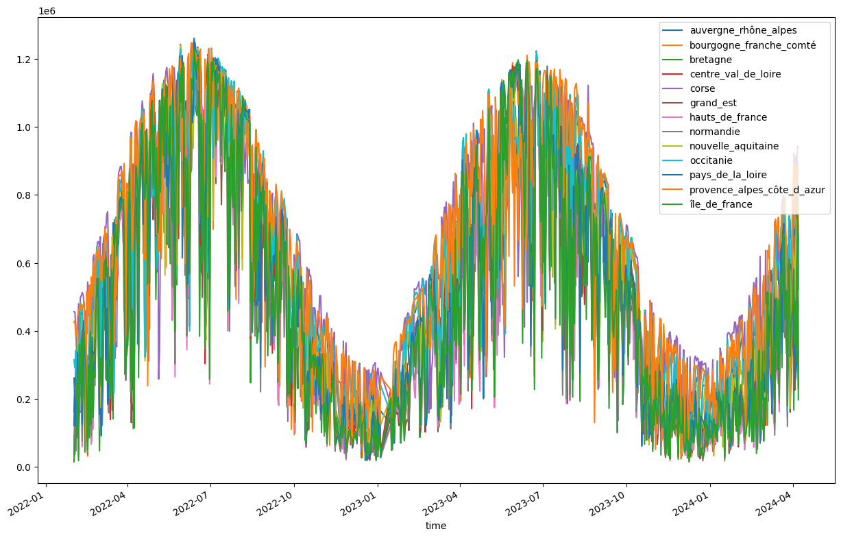
filename_ssrd_regions = "../../data/silver/mean_daily_sun_j0.csv"
filename_energy_preduction = "../../data/rte_agg_daily_2014_2024.csv"

df_ssrd_regions = pd.read_csv(filename_ssrd_regions, parse_dates=["time"]).set_index(
    "time"
)
# sanitise the column names
region_names = [
    col.replace(" ", "_").replace("'", "_").replace("-", "_").lower()
    for col in df_ssrd_regions.columns
]
df_ssrd_regions.columns = region_names
region_names = df_ssrd_regions.columns


# Doing so to add empty rows for missing days
df_ssrd_regions.plot(figsize=(15, 10))
df_ssrd_regions["days_from_start"] = [
    (date - df_ssrd_regions.index[0]).days for date in df_ssrd_regions.index
]
df_ssrd_regions.head()

	auvergne_rhône_alpes	bourgogne_franche_comté	bretagne	centre_val_de_loire	corse	grand_est	hauts_de_france	normandie	nouvelle_aquitaine	occitanie	pays_de_la_loire	provence_alpes_côte_d_azur	île_de_france	days_from_start
time
2022-02-01	261520.851689	90775.394750	163552.580967	34723.093875	456686.957700	44975.603958	21341.962363	42435.778336	185091.563333	315764.897917	122142.333333	425822.506650	15171.129004	0
2022-02-02	197822.709267	59674.926817	225057.752062	163614.112946	455816.711071	36565.521433	66463.473763	155318.998325	240519.501958	292222.562750	244625.748700	430004.543860	73755.427321	1
2022-02-03	299190.206288	190444.998208	81208.290680	150123.865750	408849.293058	124497.688083	48622.630200	47198.020700	218038.002000	342835.312917	119590.019712	383634.419163	87619.219558	2
2022-02-04	284906.858032	131882.476333	228456.231833	92169.886950	330461.622500	87107.948417	120341.102958	164888.956167	112435.209250	238153.647625	168470.041229	390108.203765	113925.635167	3
2022-02-05	362909.540192	346769.893083	318892.106625	308881.768208	310414.561742	243847.895724	259733.252833	262925.207583	402942.371958	325491.808458	338302.897500	442079.500878	274746.580333	4

df_energy_preduction = pd.read_csv(filename_energy_preduction, index_col=0)[["Solaire"]]
df_energy_preduction.index = pd.to_datetime(df_energy_preduction.index)
df_energy_preduction.head(), df_energy_preduction.tail()

(            Solaire
 Date
 2015-01-01  11370.5
 2015-01-02   8297.5
 2015-01-03   5860.5
 2015-01-04   6926.0
 2015-01-05   9786.5,
             Solaire
 Date
 2024-04-04  76581.5
 2024-04-05  72847.5
 2024-04-06  61577.5
 2024-04-07  46718.5
 2024-04-08  26677.0)

# align the indexes of the two dataframes
data = pd.concat([df_ssrd_regions, df_energy_preduction], join="inner", axis=1)
data.head()

	auvergne_rhône_alpes	bourgogne_franche_comté	bretagne	centre_val_de_loire	corse	grand_est	hauts_de_france	normandie	nouvelle_aquitaine	occitanie	pays_de_la_loire	provence_alpes_côte_d_azur	île_de_france	days_from_start	Solaire
2022-02-01	261520.851689	90775.394750	163552.580967	34723.093875	456686.957700	44975.603958	21341.962363	42435.778336	185091.563333	315764.897917	122142.333333	425822.506650	15171.129004	0	21938.5
2022-02-02	197822.709267	59674.926817	225057.752062	163614.112946	455816.711071	36565.521433	66463.473763	155318.998325	240519.501958	292222.562750	244625.748700	430004.543860	73755.427321	1	21271.0
2022-02-03	299190.206288	190444.998208	81208.290680	150123.865750	408849.293058	124497.688083	48622.630200	47198.020700	218038.002000	342835.312917	119590.019712	383634.419163	87619.219558	2	20527.5
2022-02-04	284906.858032	131882.476333	228456.231833	92169.886950	330461.622500	87107.948417	120341.102958	164888.956167	112435.209250	238153.647625	168470.041229	390108.203765	113925.635167	3	19051.0
2022-02-05	362909.540192	346769.893083	318892.106625	308881.768208	310414.561742	243847.895724	259733.252833	262925.207583	402942.371958	325491.808458	338302.897500	442079.500878	274746.580333	4	41271.5

from statsmodels.formula.api import ols

# split test for time series
from sklearn.model_selection import TimeSeriesSplit

Modeling

4 models are tested : - Only Total sun flux (no region details) - Only regions sun flux (no time feature) - Total sun flux + time - Regions sun flux + time

The Time feature allows to model a trend in the number of installed solar pannels.

exo_vars = df_ssrd_regions.columns
exo_vars = exo_vars.drop("days_from_start")
data["mean_sun"] = data[exo_vars].mean(axis=1)
endog_var = "Solaire"

tscv = TimeSeriesSplit(n_splits=60, test_size=1)  # testing on 1 days forcast

def test_model(formula="Solaire ~ mean_sun -1"):
    mod_1_mape = []
    for i, (train_index, test_index) in enumerate(tscv.split(data)):
        model_1 = ols(formula, data=data.iloc[train_index]).fit()
        if i == 0:
            first_test_index = test_index
            first_model_1 = model_1
        predictions = model_1.predict(data.iloc[test_index])
        error = data.iloc[test_index]["Solaire"] - predictions
        mape = (error.abs() / data.iloc[test_index]["Solaire"]).mean()
        mod_1_mape.append(mape)
    last_test_index = test_index
    last_model_1 = model_1
    return mod_1_mape, first_test_index, first_model_1, last_test_index, last_model_1


mod_1_mape, first_test_index, first_model_1, last_test_index, last_model_1 = (
    test_model()
)

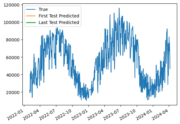
ax = data.plot(y="Solaire", label="True")
first_model_1.predict(data.iloc[first_test_index]).plot(
    ax=ax, label="First Test Predicted"
)
last_model_1.predict(data.iloc[last_test_index]).plot(
    ax=ax, label="Last Test Predicted", lw=2
)

ax.legend()

<matplotlib.legend.Legend at 0x7fccc45d9de0>

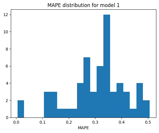
fig, ax = plt.subplots()
ax.hist(mod_1_mape, bins=20)
ax.set_title("MAPE distribution for model 1")
ax.set_xlabel("MAPE")

Text(0.5, 0, 'MAPE')

formula_2 = f"Solaire ~ {' + '.join(exo_vars)} -1"
print(formula_2)
mod_2_mape, first_test_index, first_model_2, last_test_index, last_model_2 = test_model(
    formula_2
)

Solaire ~ auvergne_rhône_alpes + bourgogne_franche_comté + bretagne + centre_val_de_loire + corse + grand_est + hauts_de_france + normandie + nouvelle_aquitaine + occitanie + pays_de_la_loire + provence_alpes_côte_d_azur + île_de_france -1

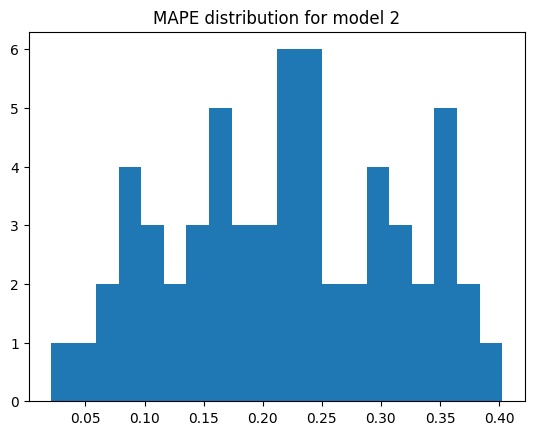
fig, ax = plt.subplots()
ax.hist(mod_2_mape, bins=20)
ax.set_title("MAPE distribution for model 2")

Text(0.5, 1.0, 'MAPE distribution for model 2')

formula_3 = "Solaire ~ mean_sun + days_from_start -1"
mod_3_mape, first_test_index, first_model_3, last_test_index, last_model_3 = test_model(
    formula_3
)
formula_4 = f"Solaire ~ {' + '.join(exo_vars)} + days_from_start -1"
mod_4_mape, first_test_index, first_model_4, last_test_index, last_model_4 = test_model(
    formula_4
)
print("formula_3", formula_3)
print("formula_4", formula_4)

formula_3 Solaire ~ mean_sun + days_from_start -1
formula_4 Solaire ~ auvergne_rhône_alpes + bourgogne_franche_comté + bretagne + centre_val_de_loire + corse + grand_est + hauts_de_france + normandie + nouvelle_aquitaine + occitanie + pays_de_la_loire + provence_alpes_côte_d_azur + île_de_france + days_from_start -1

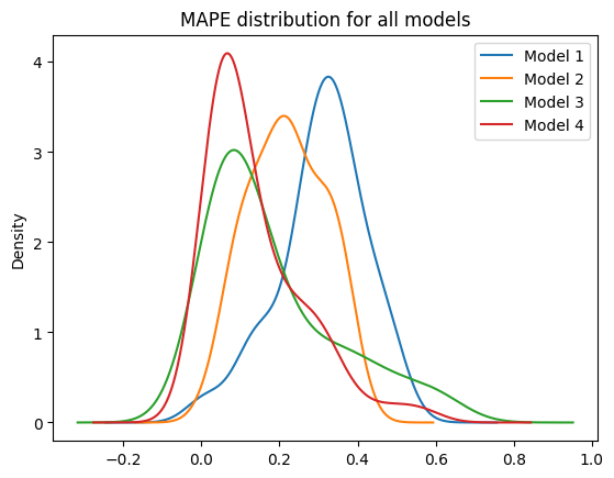
# display the MAPE distribution for all models (KDE)
fig, ax = plt.subplots()
for i, mape in enumerate([mod_1_mape, mod_2_mape, mod_3_mape, mod_4_mape]):
    pd.Series(mape).plot.kde(ax=ax, label=f"Model {i+1}")
ax.set_title("MAPE distribution for all models")
ax.legend()

<matplotlib.legend.Legend at 0x7fcc834ec7c0>

# print mean MAPE for all models
for i, mape in enumerate([mod_1_mape, mod_2_mape, mod_3_mape, mod_4_mape]):
    print(f"Model {i+1} mean MAPE: {np.mean(mape):.2%}")

Model 1 mean MAPE: 30.85%
Model 2 mean MAPE: 21.88%
Model 3 mean MAPE: 18.18%
Model 4 mean MAPE: 13.79%

Conclusion

The model performances doesn’t really follow the expected order (more feature => better performance)

Maybe this is due to some sort of over-fitting, even thought there are not so mainy features…

last_model_2.params.to_csv("sun_model_2_params.csv")