Accessing the Forecasted value of the electrical consumption

Introduction

The French Electricity Network (RTE) provides a several datasets on the electrical consumption in France.

Here, we access the forecasted value of the electrical consumption in France. The forecasted value is provided for the next 9 days.

RTE API

The API used in the consumption API.

You need an OAuth2 token to access the data. You can get one by the follwoing steps:

1. Create an account

2. Create an application

3. Add the Consumption API to the application

4. On the Application page, open your application

5. Use to button to Copy the base 64 encoded string.

Accessing the data

You can access the data by using the following code. You need to use the base64 encoded string as the secret variable.

import pandas as pd
from energy_forecast.consumption_forecast import PredictionForecastAPI

secret_file = "../../.env"
with open(secret_file, "r") as f:
    secret = f.readline().split("=", 1)[1]

prediction_forecast = PredictionForecastAPI(secret=secret)
data = prediction_forecast.get_weekly_forecast(
    start_date=pd.Timestamp.now() - pd.Timedelta(days=2),
)
data.info()

<class 'pandas.core.frame.DataFrame'>
DatetimeIndex: 288 entries, 2024-06-22 00:00:00+02:00 to 2024-06-27 23:30:00+02:00
Data columns (total 2 columns):
 #   Column                 Non-Null Count  Dtype
---  ------                 --------------  -----
 0   predicted_consumption  288 non-null    int64
 1   predicted_at           288 non-null    datetime64[ns, UTC+02:00]
dtypes: datetime64[ns, UTC+02:00](1), int64(1)
memory usage: 6.8 KB

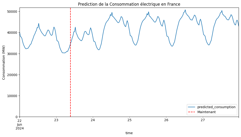
ax = data.plot(y="predicted_consumption", figsize=(12, 6))
ax.set_ylim(0)
ax.set_ylabel("Consommation (MW)")
ax.set_title("Prediction de la Consommation électrique en France")

ax_xpos = pd.Timestamp.now().timestamp() / 60
ax.axvline(ax_xpos, color="red", linestyle="--", label="Maintenant")
ax.legend()

<matplotlib.legend.Legend at 0x7fc4c12c5450>

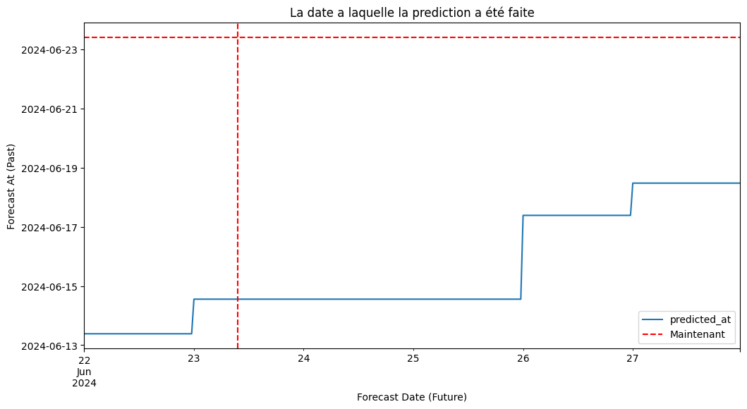
ax = data.plot(y="predicted_at", figsize=(12, 6))
ax.set_ylabel("Forecast At (Past)")
ax.set_xlabel("Forecast Date (Future)")
ax.set_title("La date a laquelle la prediction a été faite")

ax_xpos = pd.Timestamp.now().timestamp() / 60
ax.axvline(ax_xpos, color="red", linestyle="--", label="Maintenant")
ax_ypos = pd.Timestamp.now().timestamp() / 60 / 60 / 24
ax.axhline(ax_ypos, color="red", linestyle="--")
ax.legend()

<matplotlib.legend.Legend at 0x7fc4bdbbcf40>